the plotmechanic

Tales of a budding R programmer

Read this first

Gradient Descent Algorithm for Linear Regression

For this exercise I will use the data-set from this blogpost and compare the results to those of the lm() function used to calculate the linear model coefficients therein.

To understand the underlying math for the gradient descent algorithm, turn to page 5 of these notes, from Prof. Andrew Ng.

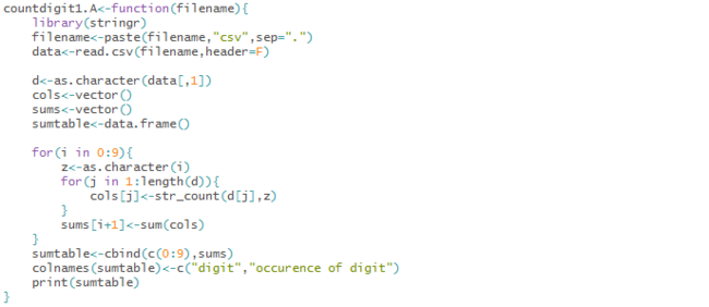
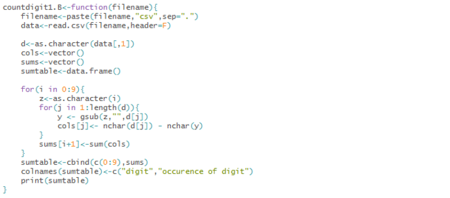
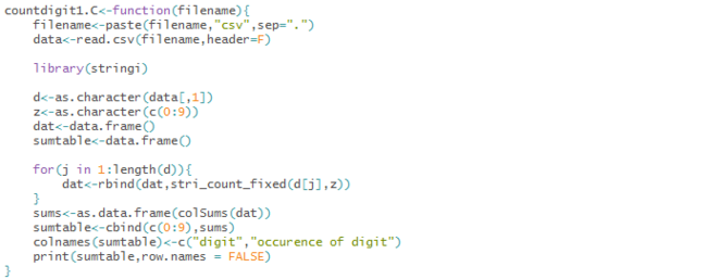
Here’s the code that automates the algorithm:

alligator = data.frame(
    lnLength = c(3.87, 3.61, 4.33, 3.43, 3.81, 3.83, 3.46, 3.76,
                 3.50, 3.58, 4.19, 3.78, 3.71, 3.73, 3.78),
    lnWeight = c(4.87, 3.93, 6.46, 3.33, 4.38, 4.70, 3.50, 4.50,
                 3.58, 3.64, 5.90, 4.43, 4.38, 4.42, 4.25)
)
X<-as.matrix(alligator$lnLength)
X<-cbind(1,X)
y<-as.matrix(alligator$lnWeight)
theta <- matrix(c(0,0), nrow=2)
alpha <- 0.1
for(i in 1:100000){
    theta_n<-theta-alpha*(t(X)%*%((X%*%theta)-y))/length(y)
    theta<-theta_n    
}

Here’s the output of the gradient descent...

Continue reading →


Normalization of data

In this post, I will cover two of the most popular techniques for normalization of data. Normalization is a very important data pre-processing step for improving performance of many machine learning algorithms.

For this purpose we will use the popular ‘Iris’ dataset. We will load the dataset from the ‘datasets’ package by using the command : data(iris). Next up, we will assign this data to another dataframe called data, which will save the normalized data points as we move through the code.

Z-score normalization:
In this method, the features are rescaled so that they have the properties of a standard normal distribution with the mean equal to zero and unit variance around the mean. The resultant values are more commonly known as z-scores and are computed as follows:
z-score.png
Here’s the R code:

data(iris)
data<-iris
for(i in 1:nrow(iris)){
...

Continue reading →


Iris Data-set : Discriminant Analysis bit by bit using R

Linear Discriminant Analysis is a useful dimensionality reduction technique with varied applications in pattern classification and machine learning. In this post, I will try to do an R replica of the Python implementation by Sebastian Raschka in this blogpost.

Following Sebastian’s footsteps, I will use the Iris dataset.

The following plots give us a crude picture of how data-points under each of the three flower categories are distributed:
iris.png
The inference we can make from the above plots is that petal lengths and petal widths could probably be potential features that could help us discriminate between the three flower species. Data-sets in the business world would usually be high-dimensional and such a simple glance at histograms might now serve our purpose.

Here’s the R code for doing the above plot:

data(iris)
library(ggplot2)
plot1 <- ggplot(iris, aes(x=Sepal.Length))
plot1<-
...

Continue reading →


Counting occurrences of digits(0-9) in a set of numbers

Last Friday, I had a conversation with a data scientist and he posed this programming question to me: “Count the number of occurrences of each of the digits 0-9 in a given set of numbers”. At first, the problem sounds simple, but given the multiple ways with which it can be solved, makes it very very interesting and a good learning experience.

I am sure there are many methods to solving this problem, but here’s my 2 cents.

Approach 1 : Convert the numbers to strings

1.A : Using ‘str_count’ function
1.A.png
View above code as text

1.B : Using ‘gsub’ and ‘nchar’ functions
1.B.png
View above code as text

1.C : Using ‘stri_count_fixed’ function
1.C.png
View above code as text

Approach 2 : Leaving the numbers as numeric

Approach 2.png
View above code as text

Moving right along, let’s do a performance evaluation of each of these methods. Here’s a snippet code that can help us calculate time taken for the data to...

Continue reading →


US Trade Deficits: A Change Point Analysis

While I was researching on ‘outlier detection’ techniques last week, I stumbled upon this well explained article on Change Point analysis.

Change Point analysis can be used to detect extreme/subtle changes in a time series and I decided to try writing the algorithm in R, starting with the case of Single Change Point Detection, before jumping onto the general case of multiple.

I borrowed the following data from here:

table_2.png

Following the article’s method, the function would primarily have three parts:

  1. Calculating the cumulative sums(CUSUM)
  2. Bootstrapping, to confirm a change
  3. Using the CUSUM Estimator to detect when the change occured

Here’s the R function:
code.png

The below image shows output from the first part of the function i.e. calculating the cumulative sums, as a grey line overlayed on the orange line which depicts the original time series of trade deficits.

New1_2.png

Moving right along, the...

Continue reading →


The News-Vendor Problem: Discrete Demand Case

Last Sunday, I came across very interesting articles and applications of the News-vendor problem and decided to write R code to automate various cases of the same. Here is a start.

In the simplest category of the News-vendor problem, such as the one outlined in this article by Prof. Evan L. Porteus, the demand is assumed to be discrete. The professor explains how the optimal amount to be ordered is the one that yields the highest expected return, which can be calculated by marginal analysis.

Here is a snippet function written in R, that automates marginal analysis for the discrete demand case of the News-vendor problem:

Code1.png

Here is how Tyler’s data looks like:

data2.png

Let’s run this function for Tyler’s case and see what the output looks like.

output2.png

The optimal solution from the DiscreteNewsVendorA function gives the solution as expected!

Sanket

Continue reading →


Creating hierarchy out of ‘n’ categorical columns

Here is an R snippet that helps converting a data frame with multiple columns into a hierarchical format.

Image 1_smallfont.png

In the below image, the right hand side table is the output achieved with the rootify function which uses the left hand side table as input. All we provide to rootify is the name of the .csv file which has the data table to be converted into the required format.

Image 2.png

The raw data as generated by rootify is valuable when it is further processed inside the arcdiagram/d3Network packages for easier and quicker data exploration. I will cover this in a future post.

Sanket

Continue reading →