Iris Data-set : Discriminant Analysis bit by bit using R

Linear Discriminant Analysis is a useful dimensionality reduction technique with varied applications in pattern classification and machine learning. In this post, I will try to do an R replica of the Python implementation by Sebastian Raschka in this blogpost.

Following Sebastian’s footsteps, I will use the Iris dataset.

The following plots give us a crude picture of how data-points under each of the three flower categories are distributed:

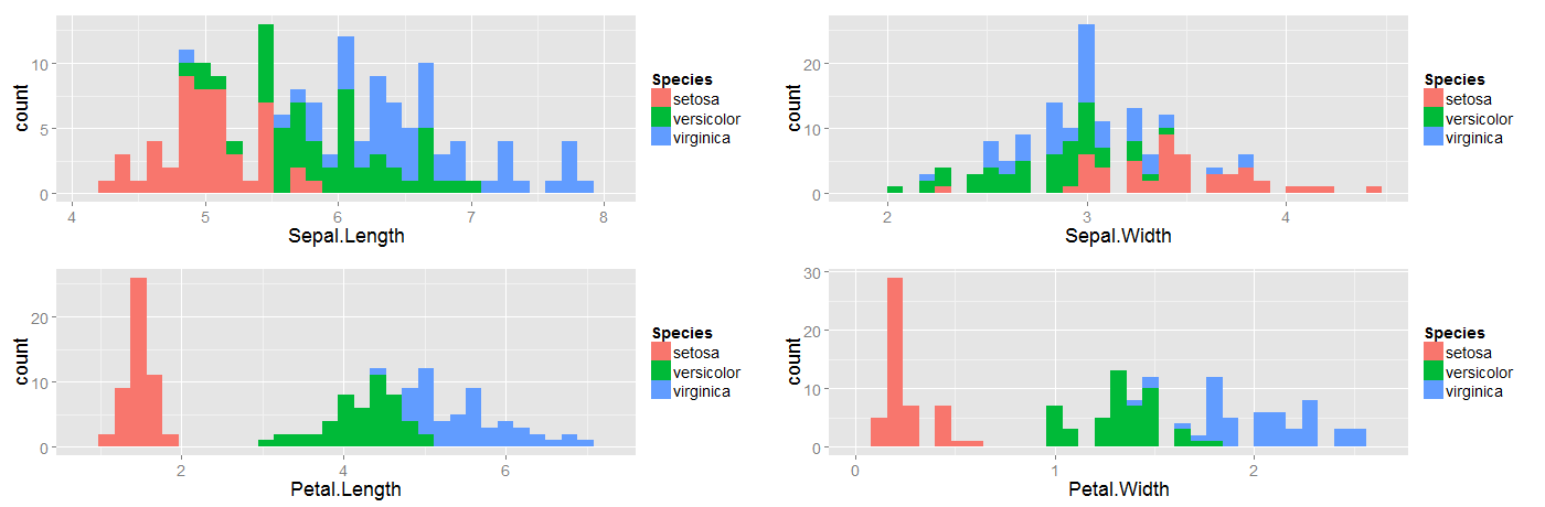
The inference we can make from the above plots is that petal lengths and petal widths could probably be potential features that could help us discriminate between the three flower species. Data-sets in the business world would usually be high-dimensional and such a simple glance at histograms might now serve our purpose.

Here’s the R code for doing the above plot:

data(iris)
library(ggplot2)
plot1 <- ggplot(iris, aes(x=Sepal.Length))
plot1<- plot1 + geom_histogram(aes(fill = Species))

plot2 <- ggplot(iris, aes(x=Sepal.Width))
plot2<- plot2 + geom_histogram(aes(fill = Species))

plot3 <- ggplot(iris, aes(x=Petal.Length))
plot3<- plot3 + geom_histogram(aes(fill = Species))

plot4 <- ggplot(iris, aes(x=Petal.Width))
plot4<- plot4 + geom_histogram(aes(fill = Species))

theme_set(theme_gray(base_size = 18))
library(gridExtra)
png("iris.png",width = 1400, height = 460, units = "px") 
m<-grid.arrange(plot1,plot2, plot3,plot4, ncol=2)
print(m)
dev.off()

To standardize the data we will use Min-Max scaling which I covered in a previous blog-post. Nonetheless, here’s the R code:

iris$Num_Species<-factor(iris$Species,labels=c(1,2,3))
data<-iris
for(i in 1:nrow(iris)){
    data$Sepal.Length[i]<-(data$Sepal.Length[i]-min(iris$Sepal.Length))/(max(iris$Sepal.Length)-min(iris$Sepal.Length))
    data$Sepal.Width[i]<-(data$Sepal.Width[i]-min(iris$Sepal.Width))/(max(iris$Sepal.Width)-min(iris$Sepal.Width))
    data$Petal.Length[i]<-(data$Petal.Length[i]-min(iris$Petal.Length))/(max(iris$Petal.Length)-min(iris$Petal.Length))
    data$Petal.Width[i]<-(data$Petal.Width[i]-min(iris$Petal.Width))/(max(iris$Petal.Width)-min(iris$Petal.Width))
}

And now, LDA in 5 steps…

1. Computing the mean vectors:

avg1<-c(mean(data[data$Num_Species==1,]$Sepal.Length),mean(data[data$Num_Species==1,]$Sepal.Width),mean(data[data$Num_Species==1,]$Petal.Length),mean(data[data$Num_Species==1,]$Petal.Width))
avg2<-c(mean(data[data$Num_Species==2,]$Sepal.Length),mean(data[data$Num_Species==2,]$Sepal.Width),mean(data[data$Num_Species==2,]$Petal.Length),mean(data[data$Num_Species==2,]$Petal.Width))
avg3<-c(mean(data[data$Num_Species==3,]$Sepal.Length),mean(data[data$Num_Species==3,]$Sepal.Width),mean(data[data$Num_Species==3,]$Petal.Length),mean(data[data$Num_Species==3,]$Petal.Width))

2. Computing the Scatter Matrices:

Next up, we will compute the two 4X4- dimensional matrices: the ‘within class’(S2 in R code) and the ‘between-class’(S_b in R code) scatter matrix, using the following R code:

S1<-matrix(0, nrow = 4, ncol = 4)
m2<-rbind(avg1,avg2,avg3)
m<-colMeans(m2)
S_bo<-matrix(0, nrow = 4, ncol = 4)
g<-unique(data$Num_Species)
for(i in 1:length(g)){
    So<-matrix(0, nrow = 4, ncol = 4)
    avg<-c(mean(data[data$Num_Species==g[i],]$Sepal.Length),mean(data[data$Num_Species==g[i],]$Sepal.Width),mean(data[data$Num_Species==g[i],]$Petal.Length),mean(data[data$Num_Species==g[i],]$Petal.Width))
    intfil1<-subset(data,data$Num_Species==g[i])
    matrix<-data.matrix(intfil1[,c(1:4)],rownames.force=NA)
    colnames(matrix)<-NULL
    for(j in 1:nrow(matrix)){
        S<-So + (matrix[j,]-avg)%*%t(matrix[j,]-avg)
        So<-S
    }
    S2<-S1+S
    S1<-S2

    S_b<-S_bo + N*(avg-m)%*%t(avg-m)
    S_bo<-S_b
}

Here are the outputs:

> S2
          [,1]      [,2]      [,3]      [,4]
[1,] 3.0058796 1.5775463 1.1593503 0.6533565
[2,] 1.5775463 2.9447917 0.5735028 0.8347917
[3,] 1.1593503 0.5735028 0.7820339 0.4429237
[4,] 0.6533565 0.8347917 0.4429237 1.0688542

&

> S_b
          [,1]      [,2]      [,3]      [,4]
[1,]  4.877479 -2.309336  7.780056  8.249923
[2,] -2.309336  1.969606 -4.042345 -3.981366
[3,]  7.780056 -4.042345 12.556817 13.190254
[4,]  8.249923 -3.981366 13.190254 13.960648

3. Solving the generalized eigenvalue problem:

y<-eigen(solve(S2)%*%S_b)

and it’s output:

> y
$values
[1]  3.219193e+01  2.853910e-01  9.184853e-15 -1.194087e-15

$vectors
           [,1]         [,2]       [,3]        [,4]
[1,] -0.1940935  0.008522342 -0.1623088 -0.73943569
[2,] -0.2394014  0.510239186  0.2676401 -0.03570183
[3,]  0.8442478 -0.540047456  0.7703101 -0.22048221
[4,]  0.4384750  0.669277287 -0.5555600  0.63509671

4. Selecting linear discriminants for the new feature subspace:

Sorting the eigen vectors:

>eig<-y$values[order(-y$values)]
>eig
[1]  3.219193e+01  2.853910e-01  9.184853e-15 -1.194087e-15

We see from the above output that two of the eigen values are almost negligible and thus the eigenpairs are less informative than the other two.

Choosing k eigen vectors with the largest eigenvalues:

W<-y$vectors[c(1,2),]

and the output:

> W
           [,1]        [,2]       [,3]        [,4]
[1,] -0.1940935 0.008522342 -0.1623088 -0.73943569
[2,] -0.2394014 0.510239186  0.2676401 -0.03570183

5. Transforming the samples onto the new subspace:

In this step, we will use the 2X4 dimensional matrix W to transform our data onto the new subspace using the following code:

mat<-data.matrix(data[,c(1:4)],rownames.force=NA)
colnames(mat)<-NULL
lda<-cbind(data.frame(t(ss%*%t(mat))),data$Species)
colnames(lda)<-c("ld1","ld2","species")

The below scatterplot represents the new feature subspace created using LDA:

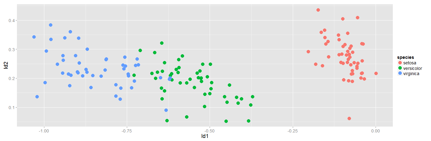
Again we see, ld1 is a much better separator of the data than ld2 is.

Sanket